Sports Analytics: College Basketball

Objective:

Understand how different statistical factors can make a college basketball team successful.

*We obtained our dataset from kaggle.com – College Basketball Dataset

Click on the button below to access R Code —> Open R Studio project & Run the code to display results & visuals

R Studio Code

We will clean the data in order to work with an accurate model. In our current database, we observe a total of 2455 variables along with 24 columns. We have data from the years 2013 to 2019. For presentation purposes, I’ll subset the database per year and use the 2019 model.

Methodology:

For the data preprocessing, we will perform the next steps:

We create a binary variable which will be WAB01 – Wins above bubble (binary).
We will insert a new column full of variables. Losses (# of games – # of wins).
Remove WAB because we made it into a binary variable. Also removed POSTSEASON and SEED due to a great number of NAs. Also, TEAM & CONF were taken out since they were strings.
We begin to check for correlation amongst variables.

*From a basketball perspective, we expect that different variables possess a high correlation with either Wins or BARTHAG (Power Ranking) since our main hypothesis is that the rest of the variables should have an impact on these 2

EX:Logically the percentage of X3P should help determine how many wins a team should have*

Now that we’ve cleaned our model and tested for correlation we’ve decided to subset our Dataset by years. Subsetting from 2013 to 2019. We will perform different subsets while also omitting NA values.

Study:

Now that we’ve subsetted by years we will start performing linear regression in order to test different models. Primarily we would like to develop at least 2 models. Both of them will use the Power Ranking (BARTHAG) as the explanatory variable but we will test the impact of the predictor “W” (Wins) in just one model.

Conclusion:

The best-fitting model for our analysis is model #2 since we found that it’s the less biased one which also possesses a great adjusted R-Squared.

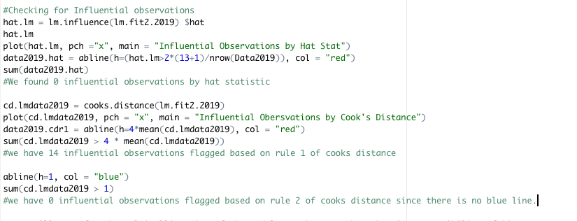
We’ll start by checking for influential observations through the hat stat and cook’s distance (2 rules)

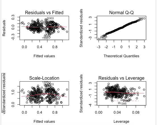
Now we’ll test for the multicollinearity of the model to make sure that there’s no possibility of bias in the selected regression model. After testing for multicollinearity we’ll begin testing for linearity of the first 2 regression models since we find these 2 to be the ones that represent the data on a more accurate way (Through Adj. R^2)

Let’s create diagnostic plots in order to make the analysis easier.

We will create training and test datasets to perform predictions and find error rates along with knn models.

Now we’ll develop more advanced visualizations, we’ll include the add-in package of ggThemeAssist which will allow us to experiment with graphs in real-time.

Our main objective was to discover which stats impact a teams success the most, which we determined was represented with 3 main stats: wins, BARTHAG (Power Ranking), and wab01 (Wins above Buble – Binary) we found shooting percentage to be a significant statistic in every model. Specifically, 2 point shooting percentage has a significant positive affect on BARTHAG, compared to three point shooting percentage. This means teams designed to shoot often and close to the basket see success more often. We also found that allowed two and three point shot percentage negatively impacts BARTHAG more than two and three point shooting percentage positively impacts BARTHAG. Overall, ADJDE, x3p_d, x2p_d, and other defense stats significantly effect a teams success. This means defense is very important to a team’s success of a team with regards to determining success.

Teams that allow a lot of shots have a very difficult time finding success.

PS: I overall enjoyed this project since it allowed me to experiment with data cleaning on a machine learning model, along with this I was able to explore new forms of visualization techniques like interactive plots through the ggiraph & trelliscope packages.

-Alfredo S.